Examples
Here are some examples what you can do with the library.
Here are some examples what you can do with the library:
These examples are just using built in functionality.
Example 1:
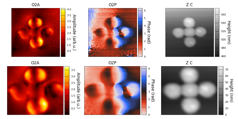
This is a comparison of the data before and after modifications, this is possible because each created image is saved in a file. In the second image modifications such as simple 3 point height leveling, cutting the data, scaling and adding a gaussian filter. This measurement was performed in transmission mode on a thin gold pentamer structur on a glass substrate.
Code
 1# Load the main functionality from the package, in this case the SnomMeasurement class.
 2from snom_analysis.main import SnomMeasurement
 3
 4# Create an instance of the SnomMeasurement class by providing the path to the measurement folder.
 5measurement = SnomMeasurement('path/to/your/measurement/folder')
 6
 7# Now you can access the data and the functions of the measurement instance.
 8# For example you can plot the data by calling the plot function.
 9# If you don't specify any arguments all channels will be plotted.
10measurement.display_channels()
11
12# You can also apply some modifications to the data, for example you can crop the data.
13# If you don't specify any arguments you will be asked to provide the cropping range using
14# some default channel and the crop will be applied to all channels.
15measurement.cut_channels()
16
17# You can also blurr the data using a gaussian filter.
18# If you want to blurr phase data you will need to have
19# the phase and amplitude channels of the same demodulation in memory.
20measurement.gauss_filter_channels_complex()
21
22# You can use a simple 3 point correction to level the height data.
23# For better leveling you can always use some other software
24# like Gwyddion and import already leveled data.
25measurement.level_height_channels_3point()
26
27# I always like to set the minimum of the height channel to zero.
28# This should be applied after the leveling. Otherwise the leveling will also change the minimum.
29measurement.set_min_to_zero(['Z C'])
30
31# Now you can plot the data again to see the modifications.
32measurement.display_channels()
33
34# You can also compare the data before and after the modifications.
35measurement.display_all_subplots()
36
37# If you are happy with the modifications you can save the data.
38# This will save the data to a new .gsf file in the measurement folder.
39measurement.save_to_gsf()
40# Per default the '_manipulated' suffix will be added to the filename,
41# to ensure you don't overwrite the original data.
Example 2:
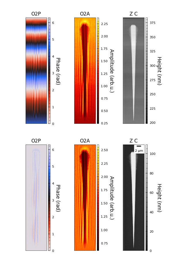
This is the data before and after some modifications such as adding a scalebar, a nonlinear correction to height, amplitude and phase, and also a phase shift to make slight phase changes more obvious. This measurement was performed in reflection mode on a thin PMMA wedge on top of a gold film. The fringes you see are an interference of the surface plasmon polaritons excited by the tip and the reflection from the PMMA edges. Due to poor AFM stability at that time the amplitude and phase data drifted quite a bit over time and need correction. Since the drifts are not linear we cannot simply use a linear correction.
Code
 1# Import filedialog to open a file dialog to select the measurement folder.
 2from tkinter import filedialog
 3
 4# Load the main functionality from the package, in this case the SnomMeasurement class.
 5from snom_analysis.main import SnomMeasurement
 6
 7# Open a file dialog to select the measurement folder.
 8directory = filedialog.askdirectory()
 9
10# It is always a good idea to select the channels you want to use before loading the data.
11channels = ['O2P', 'O2A', 'Z C']
12
13# Create an instance of the SnomMeasurement class by providing the path to the measurement folder.
14measurement = SnomMeasurement(directory, channels)
15
16# Plot the data without any modifications.
17measurement.display_channels()
18
19# You can also add a scalebar, which will be saved to the plot memory.
20measurement.scalebar(['Z C'])
21
22# for phase data the level_data_columnwise function is not yet working properly,
23# if the phase data is not in the range of 0 to 2pi (drifts more than 2pi)
24# but we can correct a linear drift in the phase data before.
25measurement.correct_phase_drift_nonlinear()
26
27# You can also aplly corrections such as a linear 2 point based y-phase drift correction.
28# measurement.correct_phase_drift()
29# or a nonlinear dift correction, wich takes into account each line and also applies
30# a linear correction in x-direction if both sides are specified
31measurement.level_data_columnwise()
32
33# I always like to set the minimum of the height channel to zero.
34# This should be applied after the drift correction.
35# Otherwise the drift correction will also change the minimum.
36measurement.set_min_to_zero(['Z C'])
37
38# You can shift the phase-offset of the phase channel.
39# Some functions will take additional parameters, if given they will apply directly.
40# If not they will promt the user with a popup window to select the parameters manually.
41measurement.shift_phase()
42# or you can specify the shift directly.
43# measurement.shift_phase(shift=0.3)
44
45# Now you can plot the data.
46measurement.display_channels()
47
48# You can also compare the data before and after the modifications.
49measurement.display_all_subplots()
Example 3:
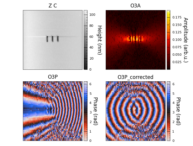
This shows the phase data before and after the synccorrection. The synccorrection gets rid of the linear phase drift caused by the movement of the lower parabola. This measurement was performed in transmission mode on a grating milled inside of a gold film. What you see is the excitation of surface plasmon polaritons propagating to the left and right of the grating.
Code
 1# Import filedialog to open a file dialog to select the measurement folder.
 2from tkinter import filedialog
 3
 4# Load the main functionality from the package, in this case the SnomMeasurement class.
 5from snom_analysis.main import SnomMeasurement, PlotDefinitions
 6PlotDefinitions.colorbar_width = 2 # colorbar width for long thin measurements looks too big
 7
 8# Open a file dialog to select the measurement folder.
 9directory = filedialog.askdirectory()
10
11# It is always a good idea to select the channels you want to use before loading the data.
12channels = ['O2P', 'O2A', 'Z C']
13
14# Create an instance of the SnomMeasurement class by providing the path to the measurement folder.
15# If we want to apply the synccorrection we need to set autoscale to False.
16measurement = SnomMeasurement(directory, channels, autoscale=False)
17
18# Plot the data without any modifications.
19measurement.display_channels()
20
21# Apply the synccorrection to the data. But we don't know the direction yet.
22# The interferometer sometimes goes in the wron direction.
23# This will create corrected channels and save them as .gsf with the appendix '_corrected'.
24measurement.synccorrection(1.6)
25
26# We want to display the corrected channels, so we reinitialize the channels with the corrected channels.
27measurement.initialize_channels(['O2P_corrected', 'O2A', 'Z C'])
28
29# Plot the corrected data.
30measurement.display_channels()
31
32# You can also compare the data before and after the modifications.
33measurement.display_all_subplots()
Example 4:
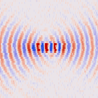
This shows a gif created from the realpart of the O3A channel and the O3P_corrected channel.
Code
 1# Import filedialog to open a file dialog to select the measurement folder.
 2from tkinter import filedialog
 3
 4# Load the main functionality from the package, in this case the SnomMeasurement class.
 5from snom_analysis.main import SnomMeasurement, PlotDefinitions
 6PlotDefinitions.colorbar_width = 4 # colorbar width for long thin measurements looks too big
 7
 8# Open a file dialog to select the measurement folder.
 9directory_name = filedialog.askdirectory()
10
11# Create an instance of the SnomMeasurement class by providing the path to the measurement folder.
12# If we want to apply the synccorrection we need to set autoscale to False.
13measurement = SnomMeasurement(directory_name, autoscale=False)
14
15# Plot the data without any modifications.
16measurement.display_channels()
17
18# Apply the synccorrection to the data. But we don't know the direction yet. The interferometer sometimes goes in the wrong direction.
19# This will create corrected channels and save them as .gsf with the appendix '_corrected'.
20# measurement.synccorrection(1.6) # for chiral coupler
21measurement.synccorrection(0.97)
22
23# We want to use the corrected channels, so we reinitialize the channels with the corrected channels.
24measurement.autoscale = True
25measurement.initialize_channels(['O2A', 'O2P_corrected'])
26
27# create a gif of the realpart of the O2A channel and the O2P_corrected channel.
28measurement.create_gif('O2A', 'O2P_corrected', frames=20, fps=10, dpi=100)
Example 5:
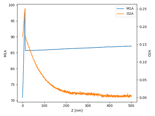
This shows basic plotting of approach curves. The data is loaded and the minimum is set to zero. The data is then displayed in a plot.
Code
 1# Import filedialog to open a file dialog to select the measurement folder.
 2from tkinter import filedialog
 3
 4# Load the main functionality from the package, in this case the SnomMeasurement class.
 5from snom_analysis.main import ApproachCurve
 6
 7# Open a file dialog to select the measurement folder.
 8directory_name = filedialog.askdirectory()
 9
10# It is always a good idea to select the channels you want to use before loading the data.
11channels = ['M1A', 'O2P', 'O2A']
12
13# Create an instance of the ApproachCurve class by providing the path to the measurement folder.
14measurement = ApproachCurve(directory_name, channels)
15
16# Set the minimum value of the data to zero.
17measurement.set_min_to_zero()
18
19# Display the channels in a plot. And scale each data set to the whole image size.
20measurement.display_channels_v2()
21
22# Alternatively you can use the display_channels() function, which will display the channels in a plot without rescaling.
23measurement.display_channels()
Example 6:
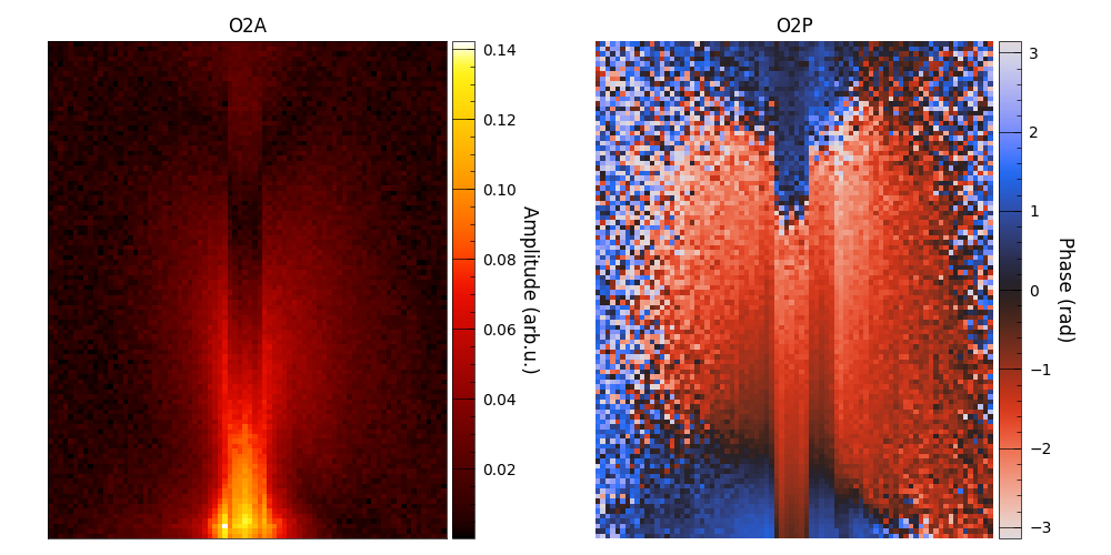
This shows basic plotting of 3D scans. The data is loaded, cutplanes are created and the minimum is set to zero. A single cutplane is then displayed in a plot. The measurement was performed on a dielectric loaded surface plasmon polariton waveguide on top of a gold film. The measurement is a cut perpendicular to the waveguide.
Code
 1# Import filedialog to open a file dialog to select the measurement folder.
 2from tkinter import filedialog
 3
 4# Load the main functionality from the package, in this case the SnomMeasurement class.
 5from snom_analysis.main import Scan3D
 6
 7# Open a file dialog to select the measurement folder.
 8directory = filedialog.askdirectory()
 9
10# It is always a good idea to select the channels you want to use before loading the data.
11channels = ['O2A', 'O2P', 'O3A', 'O3P', 'Z']
12
13# Create an instance of the Scan3D class by providing the path to the measurement folder.
14measurement = Scan3D(directory, channels)
15
16# Set the minimum value of the data to zero.
17measurement.set_min_to_zero()
18
19# Change the colorbar width to 3 on the fly will apply to all following plots.
20PlotDefinitions.colorbar_width = 3
21
22# Generate all cutplane data for the channels.
23measurement.generate_all_cutplane_data()
24
25# Match the phase offset of the channels O2P and O3P to the reference channel O2P.
26measurement.match_phase_offset(channels=['O2P', 'O3P'], reference_channel='O2P', reference_area='manual', manual_width=3)
27
28# For example display just the first cutplane of the O2P channel. Then display the first cutplane of the O3P channel.
29measurement.display_cutplane_v3(axis='x', line=0, channel='O2P')
30measurement.display_cutplane_v3(axis='x', line=0, channel='O3P')
31
32# Shift the phase of the channels O2P and O3P by an arbitrary amount to make it visually clearer what you want to see.
33measurement.shift_phase()
34
35# Display the first cutplane again with all the changes applied.
36measurement.display_cutplane_v3(axis='x', line=0, channel='O2P')
37measurement.display_cutplane_v3(axis='x', line=0, channel='O3P')
38
39# Display the real part of the first cutplane of the O2 channel and the O3 channel.
40measurement.display_cutplane_v3_realpart(axis='x', line=0, demodulation=2)
41measurement.display_cutplane_v3_realpart(axis='x', line=0, demodulation=3)
Example 7:
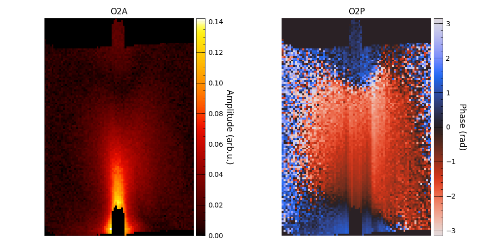
This shows basic plotting of 3D scans. The data is loaded, cutplanes are created and the minimum is set to zero. The cutplanes are then autoaligned, such that the start point of each individual approach curve is identical in z, and then displayed in a plot. This leads to a much better physical representation of the data. In this case a waveguide was in the center of the scan. This image is equivalent to the previous one but the data is shifted to align the waveguide in the center of the image.
Code
 1# Import filedialog to open a file dialog to select the measurement folder.
 2from tkinter import filedialog
 3
 4# Load the main functionality from the package, in this case the SnomMeasurement class.
 5from snom_analysis.main import Scan3D
 6
 7# Open a file dialog to select the measurement folder.
 8directory = filedialog.askdirectory()
 9
10# It is always a good idea to select the channels you want to use before loading the data.
11channels = ['O2A', 'O2P', 'O3A', 'O3P', 'Z']
12
13# Create an instance of the Scan3D class by providing the path to the measurement folder.
14measurement = Scan3D(directory, channels)
15
16# Set the minimum value of the data to zero.
17measurement.set_min_to_zero()
18
19# Change the colorbar width to 3 on the fly will apply to all following plots.
20PlotDefinitions.colorbar_width = 3
21
22# Average all individual cutplanes of the channels O2P and O3P.
23# This is an alternative approach to generating individual cutplanes.
24# All other functions will work with the averaged data, just make shure to use the 'line=0' parameter.
25measurement.average_data()
26
27# Match the phase offset of the channels O2P and O3P to the reference channel O2P.
28measurement.match_phase_offset(channels=['O2P', 'O3P'], reference_channel='O2P', reference_area='manual', manual_width=3)
29
30# For example display just the first cutplane of the O2P channel. Then display the first cutplane of the O3P channel.
31measurement.display_cutplane_v3(axis='x', line=0, channel='O2P')
32measurement.display_cutplane_v3(axis='x', line=0, channel='O3P')